Embryo RNA-seq Data
K-means Clustering
- Clustering with k=3
- Plot Marker Genes
Data Source
References

Embryo RNA-seq Data

time course experiment of individual Drosophila embryos
the time spans up to 12 hours in development
during this time key sex determination genes get activated
goal: distinguish which embryo is female or male

Pre-processing

alignment and count table was generated using STAR

# do not run here
module load ngs/STAR/2.5.3a
module load ngs/samtools

### STAR index directory ###
STAR_INDEX="../genome/STAR_dmel-all-chromosome-r6.17"

### GTF file ###
GTF_FILE="../genome/dmel-all-r6.17.gtf"

# STAR run
STAR \
--runThreadN 8 \
--readFilesCommand gunzip -c \
--quantMode GeneCounts \
--genomeDir ${STAR_INDEX} \
--sjdbGTFfile ${GTF_FILE} \
--readFilesIn ${FILEBASE}_1.txt.gz ${FILEBASE}_2.txt.gz \
--outFileNamePrefix ${FILEBASE}. \
--outSAMtype BAM SortedByCoordinate \
--limitBAMsortRAM 5000000000 \
--outFilterMultimapNmax 1

Annotation

annotation is derived from the same GTF (loaded as txdb)

library(AnnotationDbi)
library(GenomicFeatures)

txdb = loadDb("data_Kmeans/txdb")

my_exons <- exons(txdb)

exons.list.per.gene <- exonsBy(txdb, by="gene")
exonic.gene.sizes <- sum(width(reduce(exons.list.per.gene))) / 1000

head(exonic.gene.sizes)

## FBgn0000003 FBgn0000008 FBgn0000014 FBgn0000015 FBgn0000017 FBgn0000018 
##       0.299       5.414       5.477      11.791      12.819       1.794

Count Table

# read data from text file
my_counts <- read.table("data_Kmeans/count_table.txt", header = T, row.names = 1)

my_counts[1:6,1:8]

##              E1B  E1C  E1D  E1G  E1H  E2B  E2C  E2D
## FBgn0000003   76   15   23   23   12   68   22   14
## FBgn0000008 1395  676  875  699  439   34   23   19
## FBgn0000014    1    0    0    0    1   88   34   47
## FBgn0000015    0    0    0    0    2   19   19   11
## FBgn0000017 4222 2186 2614 2784 1523 2850 1718 2083
## FBgn0000018  908  364  515  278  253   36   15   19

dim(my_counts)

## [1] 17485    54

Filtering and Normalization

TPM normalization makes sure that samples and genes are comparable
- first normalize by exonic gene length
- second normalize by the sum of length corrected counts

# function to calculate TPM (see reference below)
countToTpm <- function(counts, effLen, scaler=1e6)
{
      rate <- log(counts) - log(effLen)
      denom <- log(sum(exp(rate)))
      exp(rate - denom + log(scaler))
}

# select genes
my_counts_Genes <- my_counts[grep("FBgn", rownames(my_counts)),]

# filter low counts
my_filter <- apply(my_counts_Genes, 1, function(x) length(x[x>20]) >= ncol(my_counts_Genes)/12)

my_counts_Filtered <- my_counts_Genes[my_filter,]

# match filtered genes and exonic gene sizes
my_genes_Filtered <- intersect(rownames(my_counts_Filtered), names(exonic.gene.sizes))

exonic.gene.sizes <- exonic.gene.sizes[names(exonic.gene.sizes) %in% my_genes_Filtered]
exonic.gene.sizes <- exonic.gene.sizes[order(names(exonic.gene.sizes))]

my_counts_Filtered <- my_counts_Filtered[rownames(my_counts_Filtered) %in% my_genes_Filtered,]
my_counts_Filtered <- my_counts_Filtered[order(rownames(my_counts_Filtered)),]

# check whether names are identical
stopifnot(identical(rownames(my_counts_Filtered), names(exonic.gene.sizes)))

# calculate TPM
my_TPM <- apply(my_counts_Filtered, 2, FUN = function(x){countToTpm(x, exonic.gene.sizes)})

# take log
log2_TPM <- log2(my_TPM+0.5)

log2_TPM[1:6,1:6]

##                    E1B       E1C       E1D       E1G        E1H        E2B
## FBgn0000003  5.4913503  4.296149  4.656480  4.753028  4.3757731 6.23310042
## FBgn0000008  5.5107778  5.589526  5.712513  5.489284  5.3727542 1.35804085
## FBgn0000014 -0.9106273 -1.000000 -1.000000 -1.000000 -0.7559121 2.53083317
## FBgn0000015 -1.0000000 -1.000000 -1.000000 -1.000000 -0.7719412 0.04186372
## FBgn0000017  5.8614745  6.035190  6.045044  6.233035  5.9183222 6.20060925
## FBgn0000018  6.4770042  6.284183  6.535293  5.749910  6.1637671 2.82643640

dim(log2_TPM)

## [1] 8983   54

K-means Clustering

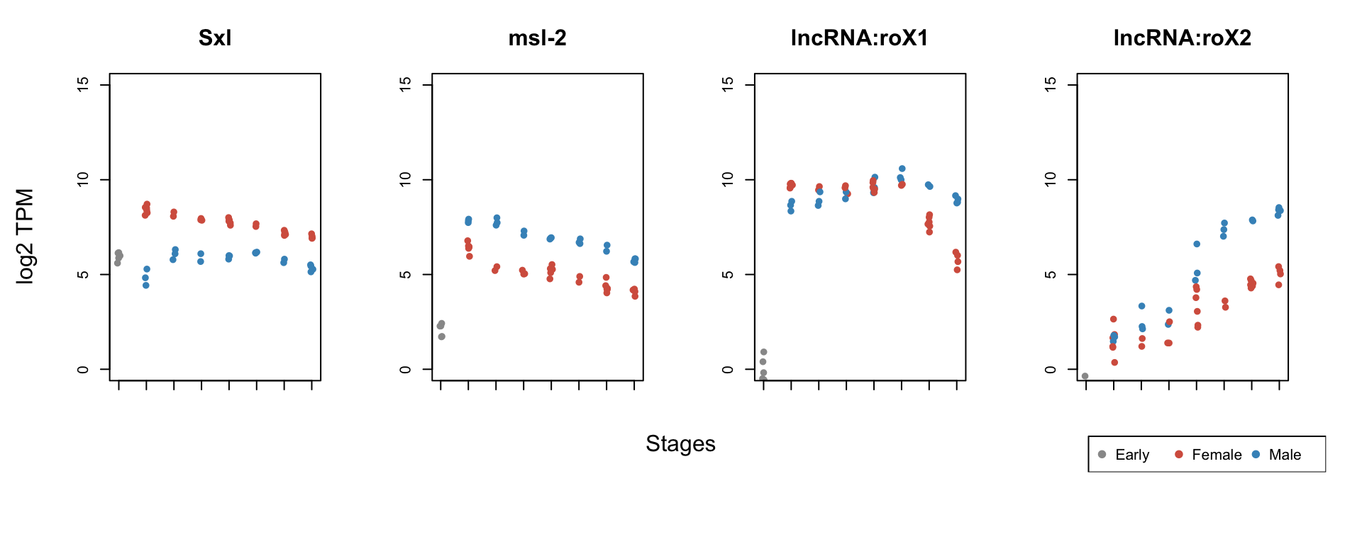
Clustering with k=3

first embryo is before sex determination is initiated
that´s why we set k = 3 (early, female and male)

library(org.Dm.eg.db)

# select well known sex-specific marker genes
my_favorite_genes <- c("Sxl", "msl-2" ,"lncRNA:roX1", "lncRNA:roX2")
names(my_favorite_genes) <- mapIds(org.Dm.eg.db, my_favorite_genes, "FLYBASE", keytype="SYMBOL", multiVals="first")

set.seed(99)

# k-means with k=3
kmeans_clusters <- kmeans(apply(log2_TPM[ rownames(log2_TPM) %in% names(my_favorite_genes), ], 1, 
                         function(x){ (x-mean(x))/sd(x) }),3, nstart=25, iter.max=1000)

my_sexes <- factor(as.integer(kmeans_clusters$cluster))

head(my_sexes)

## [1] 1 1 1 1 1 2
## Levels: 1 2 3

Plot Marker Genes

plot TPM values to see sex-specific pattern

# conditions
my_conditions <- factor(substr(colnames(log2_TPM),1,2))

# setup color
my_color_palette <- c("#999999", "#d6604d", "#4393c3")

par(mfrow=c(1,4), oma=c(4,2,0,2))

# iterate through marker genes
for(i in seq_along(my_favorite_genes)){
    
    plotDots(log2_TPM[rownames(log2_TPM) == names(my_favorite_genes)[i],], 
                     my_title = my_favorite_genes[i], 
                     color_palette = my_color_palette, 
                     color_groups = my_sexes, 
                     conditions = my_conditions, 
                     point_size = 0.8)
}

mtext(text = "Stages", side = 1, line = -2, outer = TRUE)
mtext(text = "log2 TPM", side = 2, outer = TRUE)

par(fig = c(0,1,0,1), mar=c(0,0,0,0), new = TRUE)
plot(0,0, xlab="", ylab="", xaxt="n", yaxt="n", bty="n", type="n" )
legend("bottomright", legend = c("Early", "Female", "Male"), pch = 19, col = my_color_palette, horiz = T)

Conclusions:

Expected sex-specific pattern:
- Sxl is female, whereas msl-2 male specifc
- roX1 is unspecfic until it becomes male specific
- roX2 expression is activated later only in males
Using RNA-seq expression of known sex-specific genes one can easily distinguish between female and male embryos

Data Source

The dataset was generated by Tamas Schauer (LMU, BMC, Becker group)

References

Progressive dosage compensation during Drosophila embryogenesis is reflected by gene arrangement. Prayitno K, Schauer T, Regnard C, Becker PB. EMBO Rep. 2019 Aug;20(8):e48138. doi: 10.15252/embr.201948138. Epub 2019 Jul 9. PMID: 31286660

TPM calculation: https://haroldpimentel.wordpress.com/2014/05/08/what-the-fpkm-a-review-rna-seq-expression-units/

K-Means Clustering - Female/Male Embryos