Determining NFR width by cross-correlation
Nucleosome Data by MNase-seq
- dyad coverages are centered at different kind of sites
- transcription factor (TF) motif (PWM) positions
- transcription start sites (TSS)
- TSS +1 nucleosome
- goal is to estimate the distance between flanking nucleomes surrounding the center
- this can be called NFR (nucleosome “free” region) width
- (side note: one could subtract 147 bp (1 nucleosome) from this width)
Method Description
- the method is inspired by Ocampo et al. 2016 and Chereji et al. 2018
- 2 Gaussian distributions mimic 2 flanking nucleosomes with known distance between them (theoretical pattern)
- for each site, the nucleosome signal is compared to the theoretical pattern (by cross-correlation)
- the actual distance for the given site is selected by maximizing the cross-correlation
### helper functions ###

# generate Gaussian distribution
gaussmf <- function (x, sigma, mean) {
      height <- 1
      mfVals = (height * exp(-(((x - mean)^2)/(2 * (sigma^2)))))
      mfVals
}

# create NFR-like pattern
makeNFR <- function(d, beforeRef, afterRef){

      apply(sapply(c(-0.5,0.5), function(x) {gaussmf(seq(-beforeRef, afterRef), 40, x * d)}), 1, sum)

}

# scale between minimum and maximum
scaler <- function(x, probs = c(0.01,0.99)){
      (x - quantile(x, probs[1])) / (quantile(x, probs[2])-quantile(x, probs[1]))
}


### main function ###

# iterate through each row of the matrix
# use ccf function to find maximum correlation
# pick d which corresponds to the maximum correlation

calcNFRwidth <- function(my_mat,
                          beforeRef = 200,
                          afterRef =  200,
                          mc.cores = 16){


    # here before and after is not necessarily symmetric (e.g. if matrix is not centered at NFR)
    my_mat_sub <- my_mat[, (ceiling(ncol(my_mat)/2)-beforeRef):(ceiling(ncol(my_mat)/2)+afterRef-1)]


    res <- parallel::mclapply(1:nrow(my_mat_sub), mc.cores = mc.cores, function(ridx){

        rx <- scaler(my_mat_sub[ridx, ])

        bestR <- 0
        spacingV <- NA
        shiftV <- NA

        total_width <- beforeRef+afterRef

        if(round(sd(rx), 3) != 0 & sum(is.na(rx)) == 0){

            for (d in 1:(total_width+100)) {

                # here before and after should be symmetric (left and right to center)
                y <-  makeNFR(d = d, beforeRef = total_width/2, afterRef = total_width/2)

                my_ccf <- ccf(rx,y, lag.max = 50, plot=FALSE)

                r <- max(my_ccf$acf)
                shift <- my_ccf$lag[my_ccf$acf == r]

                if (r > bestR) {
                    bestR <- r
                    shiftV <- shift
                    spacingV <- d
                }
            }

        }


        c(r = round(bestR, 2), width = spacingV, shift = shiftV)

    })

    df <- t(as.data.frame(res))
    rownames(df) <- rownames(my_mat_sub)
    return(df)

}
Budding Yeast Data #1
- in vivo MNase-seq from yeast (S.cerevisae)
- centered at putative TF sites (based on PWM)
- single end data: all fragments are considered
# load site centered matrix
load("data_NFRwidth/smooth.mat.TF.yeast.invivo.MNase.rda")
# use +/- 200 bp from the center
beforeRef <- 200
afterRef <- 200file_path <- paste0("data_NFRwidth/NFRwidth.TF.yeast.invivo.MNase.set",beforeRef,"_",afterRef,".txt")
if(file.exists(file_path)){
#read NFR data (pre-calculated)
df <- read.table(file_path, row.names = 1, header = T)
} else {
# run analysis
df <- calcNFRwidth(my_mat = my_mat,
beforeRef = beforeRef,
afterRef = afterRef)
write.table(df, file = file_path, sep = "\t", row.names = T, col.names = NA)
}
head(df)## r width shift
## 1 0.71 279 -10
## 2 0.51 112 24
## 3 0.67 421 40
## 4 0.87 1 -50
## 5 0.68 353 50
## 6 0.97 320 6- the greater the correlation the more similar is the actual pattern to the theoretical
- width indicates the NFR width
- shift indicates how far the signal had to be shifted from the center to get the max correlation
Heatmap Visualization
# heatmap  ordered by NFR width
library(RColorBrewer)

par(mfrow=c(1,1), oma=c(2,0,0,1))

plotHeatmap(mat = my_mat, df = df, plot_title = "Nucleosomes centered at TF")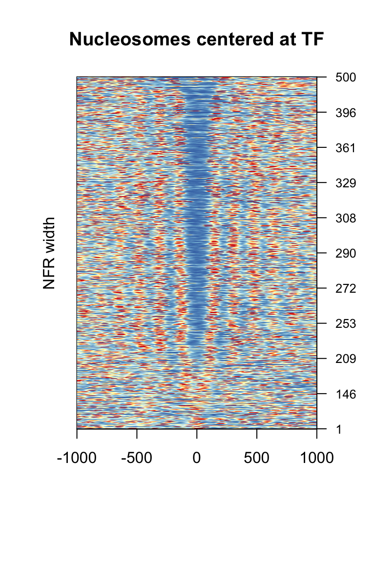
- The order on the heatmap seems to be ok
Exploring the Values
# check distributions
par(mfrow=c(1,3), oma=c(2,0,0,0))

hist(df[,1], breaks = 500, main = "NFR correlation", xlab="")
hist(df[,2], breaks = 250, main = "NFR width", xlab="")
hist(df[,3], breaks = 500, main = "NFR shift", xlab="")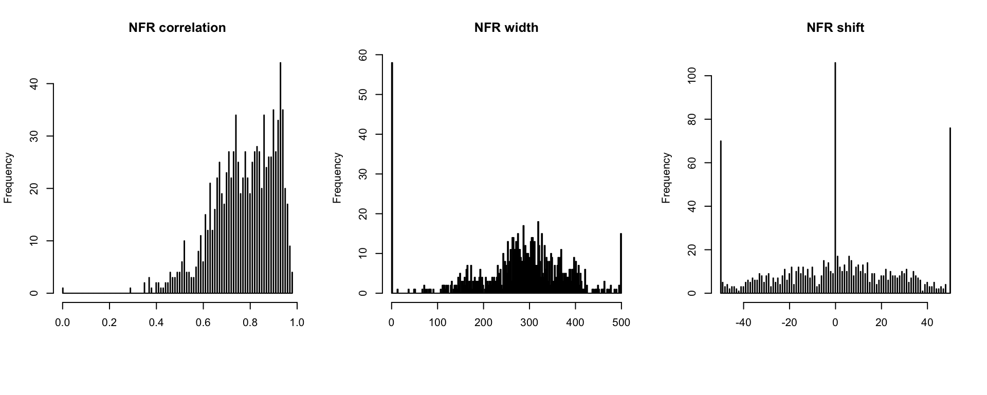
- the majority of the width values are between 200-400
- there are some values at the extremes (1, 500)
Example Sites
# choose examples by interesting values

examples <- c(which(df[,2] > 0   & df[,2] <= 1 & df[,1] > 0.9)[1],
              which(df[,2] > 165 & df[,2] <= 170 & df[,1] > 0.9)[1],
              which(df[,2] > 295 & df[,2] <= 305 & df[,1] > 0.9)[1],
              which(df[,2] > 499 & df[,2] <= 500 & df[,1] > 0.6)[1],
              which(df[,2] > 0   & df[,2] <= 1 & df[,1] < 0.7)[1],
              which(df[,2] > 165 & df[,2] <= 170 & df[,1] < 0.7)[1],
              which(df[,2] > 295 & df[,2] <= 305 & df[,1] < 0.7)[1],
              which(df[,2] > 499 & df[,2] <= 500 & df[,1] < 0.6)[1])

par(mfrow=c(2,4), oma=c(0,0,2,0))

plotExamples(examples = examples)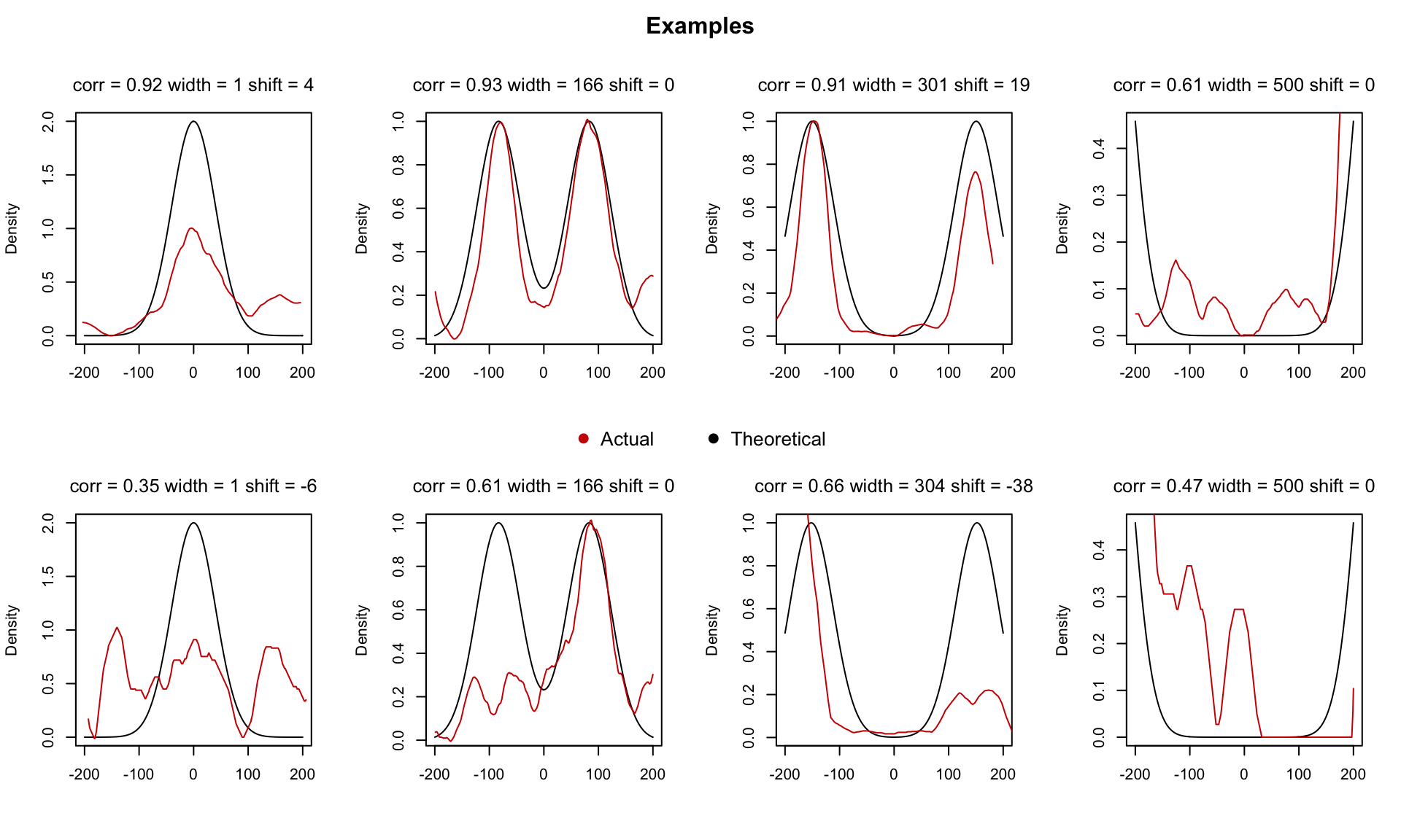
- width = 1 (no distance) means that a single nucleosome is sitting at the center
- width = 500 suggests a nucleosome is at one side only (not a real NFR?)
- lower correlation values might give a reasonable width although the pattern is more noisy
Budding Yeast Data #2
- in vivo MNase-seq from yeast (S.cerevisae)
- paired end data: mono-nuclesomal fragments are selected
- centered at TSS +1 nucleosome (which was determined previously by Chereji et al. 2018)
- this creates a problem that the matrix is not centered at the NFR
- (Side note: I could have used the NFR center positions from Chereji et al.)
- (Side note2: Chereji et al. also use a similar method where they first map the +1 and -1 nucleosomes)
- one goal is here to test different window sizes left and right
# load site centered matrix
load("data_NFRwidth/smooth.mat.plusOne.yeast.invivo.MNase.rda")
# settings are different window sizes
# windows are asymmetric as the signal is centered at the +1 nucleosome
settings <- list(c(450,50),
c(400,50),
c(350,50),
c(300,50))
for(i in seq_along(settings)){
beforeRef <- settings[[i]][1]
afterRef <- settings[[i]][2]
file_path <- paste0("data_NFRwidth/NFRwidth.plusOne.yeast.invivo.PE.MNase.set",beforeRef,"_",afterRef,".txt")
if(file.exists(file_path)){
#read NFR data (pre-calculated)
df <- read.table(file_path, row.names = 1, header = T)
assign(paste0("df",i), df)
} else {
# run analysis
df <- calcNFRwidth(my_mat = my_mat,
beforeRef = beforeRef,
afterRef = afterRef)
write.table(df, file = file_path, sep = "\t", row.names = T, col.names = NA)
assign(paste0("df",i), df)
}
}Heatmap Visualization
# heatmap  ordered by NFR width
library(RColorBrewer)

par(mfrow=c(1,4), oma=c(1,0,1,1))

# iterate through settings
for(i in seq_along(settings)){

    plotHeatmap(mat = my_mat, df = get(paste0("df",i)),
            plot_title = paste0("beforeRef = ",settings[[i]][1],"; afterRef =",settings[[i]][2]))
}

title(main = "Nucleosomes centered at TSS+1 nucleosome", outer = TRUE)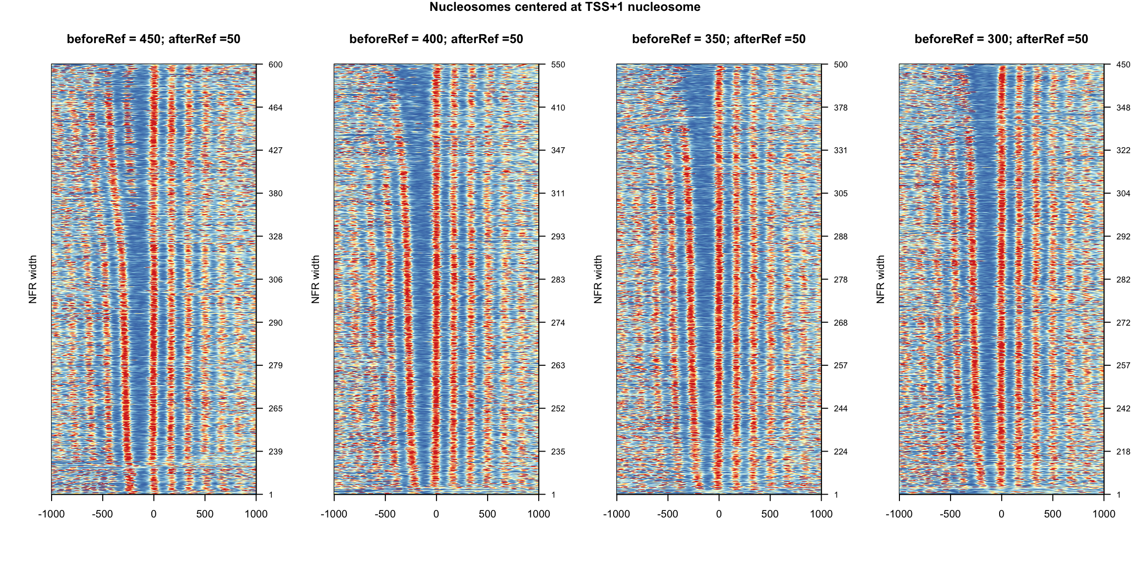
- 1st window does not capture -1 properly (there is a small nuclesome in between)
- 3rd window looks the most reasonable
Exploring the Values
# check distributions
par(mfrow=c(1,3), oma=c(2,0,0,0))

df <- df3
beforeRef = 350; afterRef = 50

hist(df[,1], breaks = 500, main = "NFR correlation", xlab="")
hist(df[,2], breaks = 250, main = "NFR width", xlab="")
hist(df[,3], breaks = 500, main = "NFR shift", xlab="")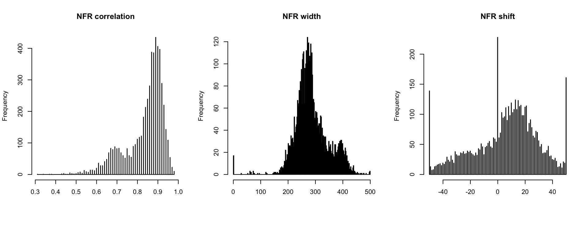
- there is a shoulder at 400 (probably because window size is limited?)
Example Sites
# choose examples by interesting values

examples <- c(which(df[,2] > 0   & df[,2] <= 1 & df[,1] > 0.8)[1],
              which(df[,2] > 150 & df[,2] <= 170 & df[,1] > 0.8)[1],
              which(df[,2] > 295 & df[,2] <= 305 & df[,1] > 0.9)[1],
              which(df[,2] > 499 & df[,2] <= 500 & df[,1] > 0.6)[2],
              which(df[,2] > 0   & df[,2] <= 1 & df[,1] < 0.7)[1],
              which(df[,2] > 165 & df[,2] <= 170 & df[,1] < 0.7)[1],
              which(df[,2] > 295 & df[,2] <= 305 & df[,1] < 0.7)[1],
              which(df[,2] > 499 & df[,2] <= 500 & df[,1] < 0.6)[1])

par(mfrow=c(2,4), oma=c(0,0,2,0))

plotExamples(examples = examples)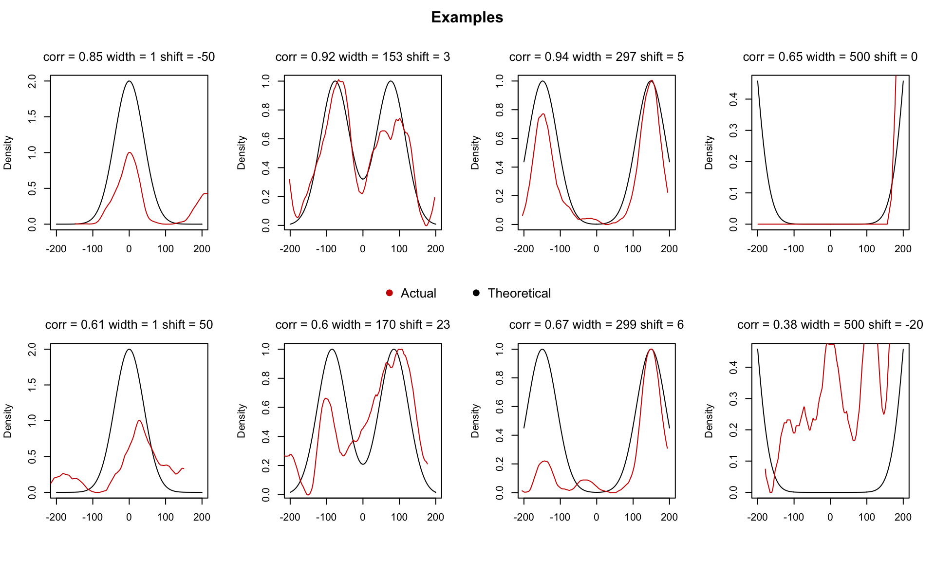
- the profiles with high correlation look quite ok
Compare to Chereji etal. data
- Chereji et al. used a different method
- they first determine -1 and +1 nucleomes positions
- they use cross-correlation to refine those positions
- they detemine NFR width (NDR width) as the distance between -1 and +1
- they substract 147 bp (1 nucleosome)
# read published data
NFR <- read.table("data_NFRwidth/13059_2018_1398_MOESM2_ESM.txt", sep = "\t", header = T, stringsAsFactors = F)

library(LSD)
par(mfrow=c(1,1), oma=c(2,2,0,2))


# merge datasets
df_NFR <- merge(df, NFR, by.x = "row.names", by.y = "ORF")

# add 147 for comparison
heatscatter(df_NFR$width, df_NFR$NDR.Width+147,
            xlab = "cross-correlation method", ylab = "Chereji method",
            main = "Comparison", pch=19, cex=0.6,
            xlim = c(100,600), ylim = c(100,600))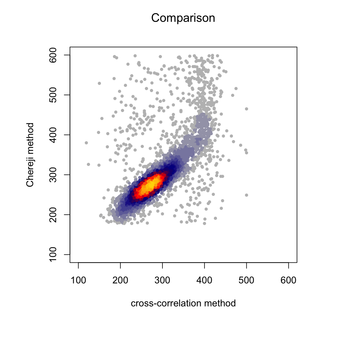
- there is a good match for NFRs between 200-400
- the limit at 400 is visible here as well
Heatmap Visualization
# heatmap  ordered by NFR width
par(mfrow=c(1,2), oma=c(1,0,1,1))

my_mat <- my_mat[rownames(my_mat) %in% df_NFR$Row.names,]
my_mat <- my_mat[order(rownames(my_mat)),]

identical(as.character(df_NFR$Row.names), rownames(my_mat))
## [1] TRUEdf <- df_NFR[,c(2,3,4)]
rownames(df) <- df_NFR$Row.names
plotHeatmap(mat = my_mat, df = df, plot_title = "cross-correlation method")
df <- df_NFR[,c(2,14,4)]
rownames(df) <- df_NFR$Row.names
plotHeatmap(mat = my_mat, df = df, plot_title = "Henikoff method")
title(main = "Nucleosomes centered at TSS+1 nucleosome", line = -0.5, outer = TRUE)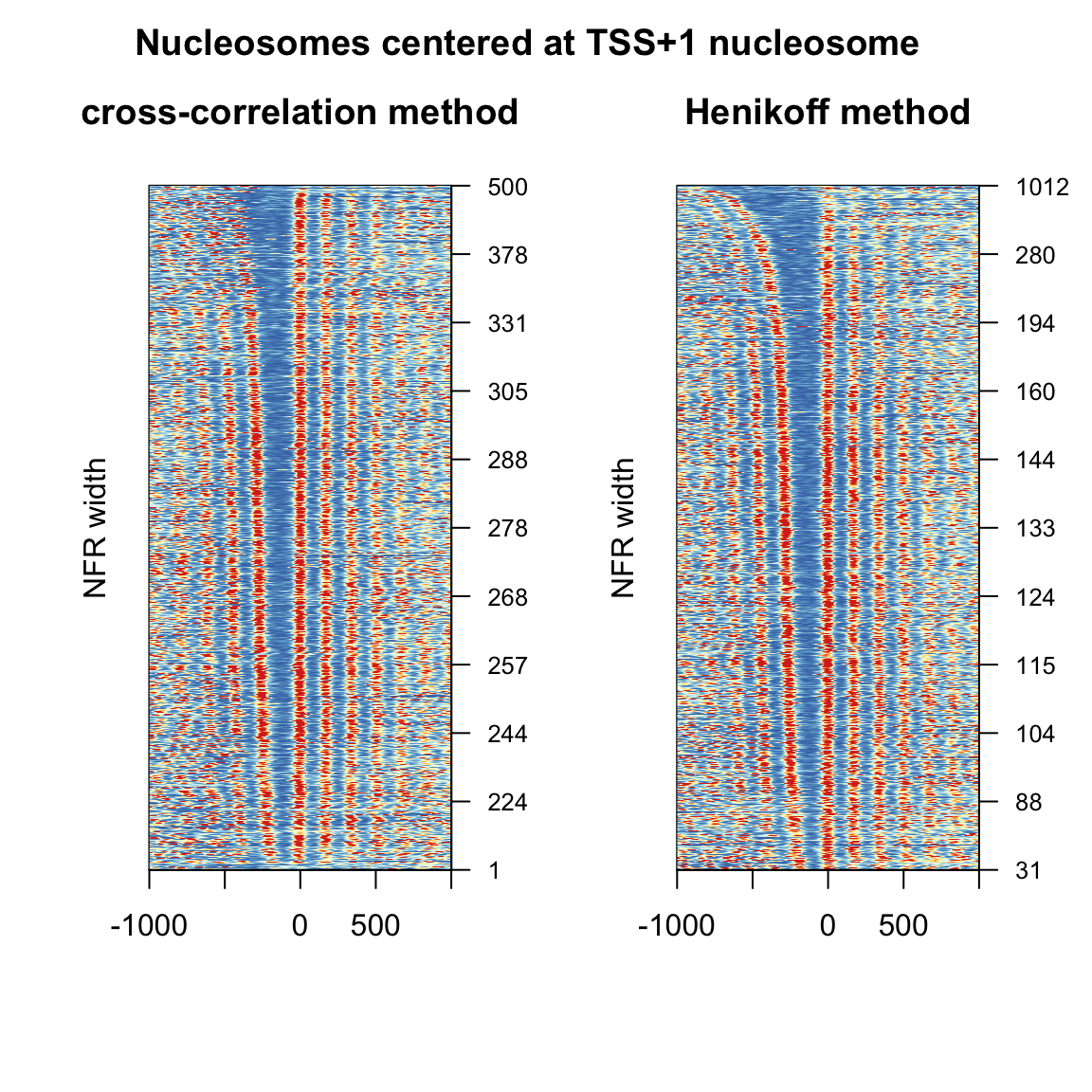
Conclusions:
- NFR width up to the window limit matches published results
- longer NFRs are not captured well with this method
using larger window sizes is not an option (small nucleosome appears in the middle)
- the method can be still useful in the first example when centered at TF motif
in this case the nucleosome might be exactly at the TF center (which results in a width=1)
Data Source
The first dataset was generated by Elisa Oberbeckmann (LMU, BMC, Korber group)
The second dataset was generated by Ashish Singh (LMU, BMC, Müller-Planitz group)
References
The ISW1 and CHD1 ATP-dependent chromatin remodelers compete to set nucleosome spacing in vivo. Ocampo J, Chereji RV, Eriksson PR, Clark DJ. Nucleic Acids Res. 2016 Jun 2;44(10):4625-35. doi: 10.1093/nar/gkw068. Epub 2016 Feb 9. PMID: 26861626
Precise genome-wide mapping of single nucleosomes and linkers in vivo. Chereji RV, Ramachandran S, Bryson TD, Henikoff S. Genome Biol. 2018 Feb 9;19(1):19. doi: 10.1186/s13059-018-1398-0. PMID: 29426353