Simple Data Visualization

---

Data Types

continuous

# blood pressure
set.seed(111)
blood_pressure <- rnorm(1000, mean = 120, sd = 10)
head(blood_pressure)

## [1] 122.35221 116.69264 116.88376  96.97654 118.29124 121.40278

discrete

# cell counts in a counting chamber
set.seed(222)
cell_counts <- rpois(1000, lambda = 10)
head(cell_counts)

## [1] 14  9 14  8 10  9

categorical

# blood type of person
set.seed(333)
blood_type <- factor(sample(c("A", "B", "AB", "0"), size = 1000, replace = T))
head(blood_type)

## [1] B  A  AB B  AB 0 
## Levels: 0 A AB B

---

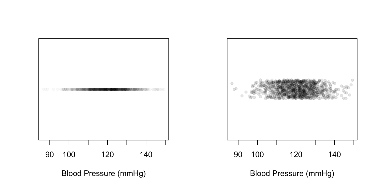
Stripcharts

par(mfrow=c(1,2))

# overplot
stripchart(blood_pressure, xlab = "Blood Pressure (mmHg)",
           pch = 19, col = rgb(0,0,0,0.025), cex=0.75, method = "overplot")

# jitter
stripchart(blood_pressure, xlab = "Blood Pressure (mmHg)",
           pch = 19, col = rgb(0,0,0,0.1), cex=0.75, method = "jitter")

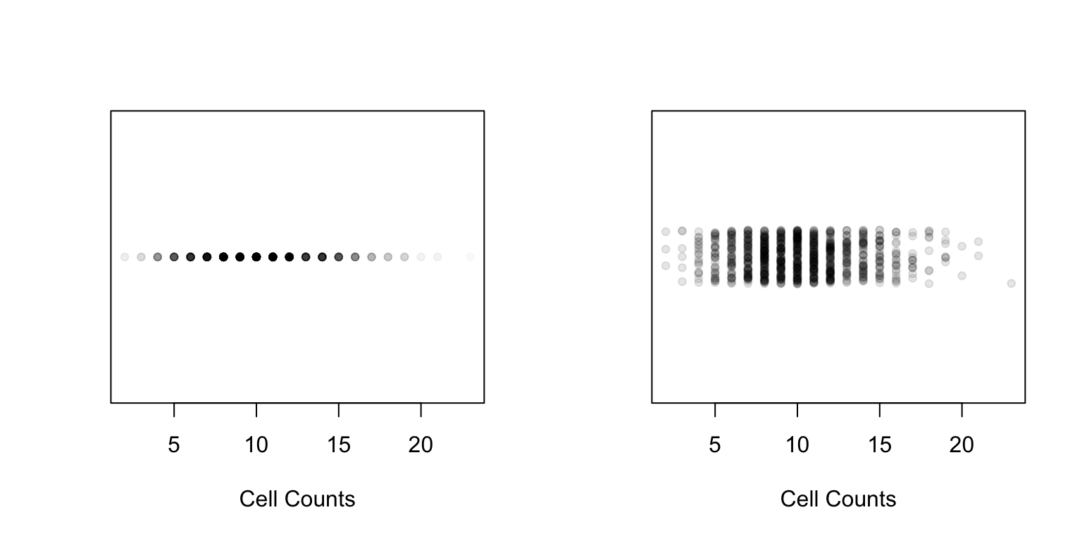
par(mfrow=c(1,2))

stripchart(cell_counts, xlab = "Cell Counts",
           pch = 19, col = rgb(0,0,0,0.025), cex=0.75, method = "overplot")

stripchart(cell_counts, xlab = "Cell Counts",
           pch = 19, col = rgb(0,0,0,0.1), cex=0.75, method = "jitter")

---

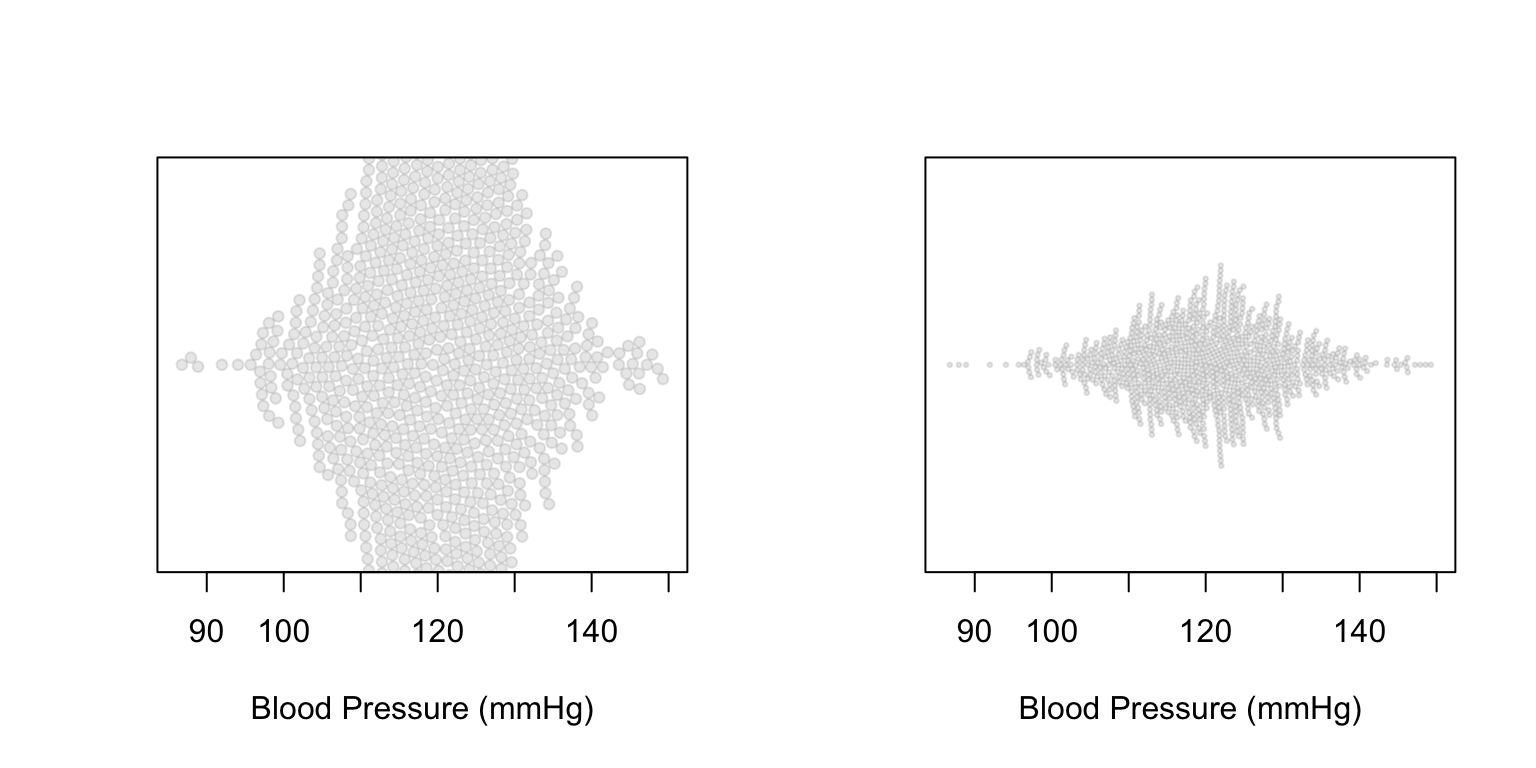
Beeswarm

library(beeswarm)

par(mfrow=c(1,2))

beeswarm(blood_pressure, xlab = "Blood Pressure (mmHg)",
         pch = 19, col = rgb(0,0,0,0.1), cex=0.75, vertical = F)

beeswarm(blood_pressure, xlab = "Blood Pressure (mmHg)",
         pch = 19, col = rgb(0,0,0,0.1), cex=0.33, vertical = F)

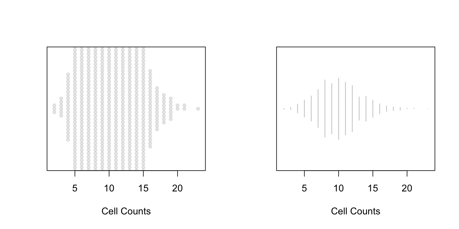
par(mfrow=c(1,2))

beeswarm(cell_counts, xlab = "Cell Counts",
           pch = 19, col = rgb(0,0,0,0.1), cex=0.75, vertical = F)

beeswarm(cell_counts, xlab = "Cell Counts",
           pch = 19, col = rgb(0,0,0,0.1), cex=0.10, vertical = F)

---

Histograms

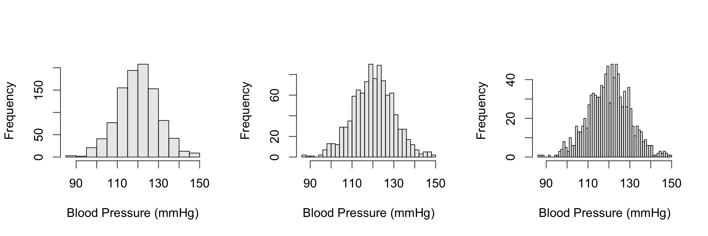
par(mfrow=c(1,3), cex=1.25)

hist(blood_pressure, xlab = "Blood Pressure (mmHg)", 
     main = "", col = rgb(0,0,0,0.1), breaks = 10)

hist(blood_pressure, xlab = "Blood Pressure (mmHg)", 
     main = "", col = rgb(0,0,0,0.1), breaks = 30)

hist(blood_pressure, xlab = "Blood Pressure (mmHg)", 
     main = "", col = rgb(0,0,0,0.1), breaks = 50)

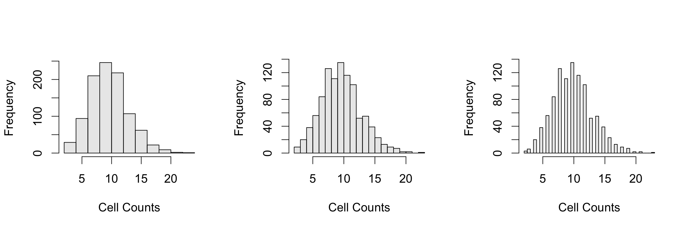
par(mfrow=c(1,3), cex=1.25)

hist(cell_counts, xlab = "Cell Counts", 
     main = "", col = rgb(0,0,0,0.1), breaks = 10)

hist(cell_counts, xlab = "Cell Counts", 
     main = "", col = rgb(0,0,0,0.1), breaks = 20)

hist(cell_counts, xlab = "Cell Counts", 
     main = "", col = rgb(0,0,0,0.1), breaks = 50)

---

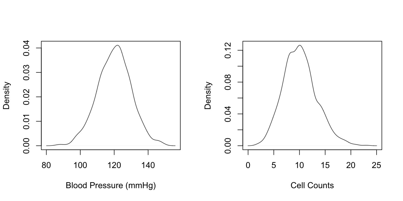
Density plots

par(mfrow=c(1,2))

plot(density(blood_pressure), xlab = "Blood Pressure (mmHg)", 
     main = "", col = rgb(0,0,0,0.8))

plot(density(cell_counts), xlab = "Cell Counts", 
     main = "", col = rgb(0,0,0,0.8))

---