Simulation
- random data from normal distribution
- set.seed for reproducibility
- seed was purposely selected to have a weak association
# set n
n <- 5000

# generate data
set.seed(285)

df <- data.frame(x = rnorm(n),
                 y = rnorm(n))

# order by x
df <- df[order(df$x),]
# plot data
par(mfrow=c(1,1))

plot(y ~ x, data = df, main = "", pch=19, col = "#00000022", xlim = c(-4,4), ylim = c(-4,4))
legend("topleft", legend = paste("r =", round(cor(df$x,df$y),2)))
legend("topright", legend = paste("pval =", format(cor.test(df$x,df$y)$p.value, digits = 2, scientific = T)))
abline(lm(y ~x, data = df), col="red3", lwd=2)
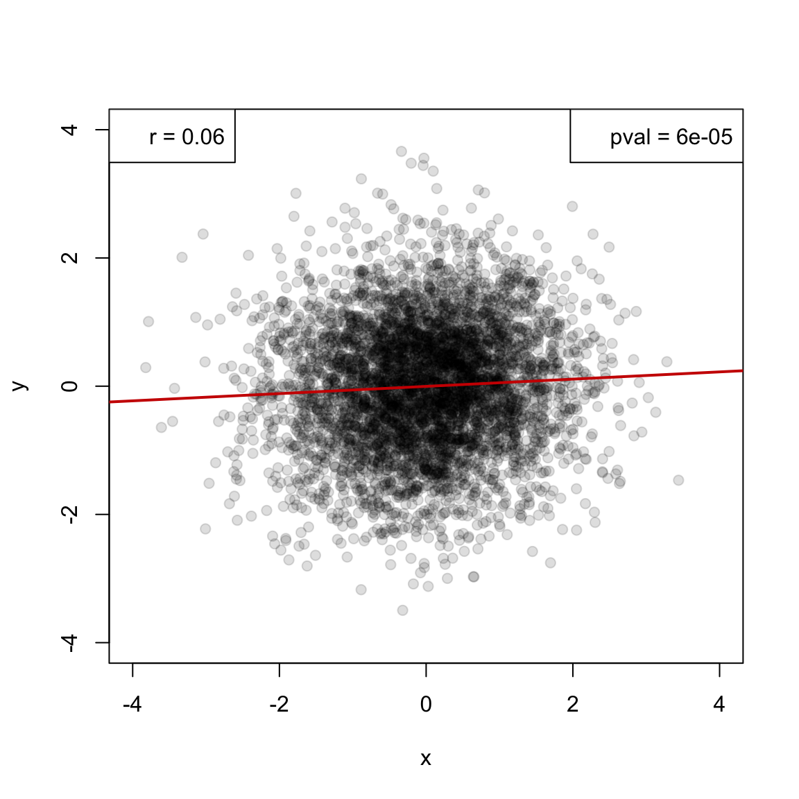
- very weak assosication
- p-value is misleading (<0.05)
Binning
- bin and average both x and y variables
par(mfrow=c(2,2), oma=c(2,2,2,2))

# plot without binning
plot(y ~ x, data = df, main = "no binning", pch=19, col = "#00000022")
legend("topleft", legend = paste("r =", round(cor(df$x,df$y),2)))
legend("topright", legend = paste("pval =", format(cor.test(df$x,df$y)$p.value, digits = 2, scientific = T)))
abline(lm(y ~x, data = df), col="red3", lwd=2)


# iterate through different number of bins
for(n_bins in c(150,50,20)){
    x_binned <- sapply(1:n_bins, FUN = function(i){  mean(df$x[((i-1)*(n/n_bins)+1):((i)*(n/n_bins))])})
    y_binned <- sapply(1:n_bins, FUN = function(i){  mean(df$y[((i-1)*(n/n_bins)+1):((i)*(n/n_bins))])})

    plot(x_binned, y_binned, main = paste("n bins =", n_bins), pch=19, col = "#00000055")
    legend("topleft", legend = paste("r =", round(cor(x_binned,y_binned),2)))
    legend("topright", legend = paste("pval =", format(cor.test(x_binned,y_binned)$p.value, digits = 2, scientific = T)))
    abline(lm(y_binned ~ x_binned), col="red3", lwd=2)
}
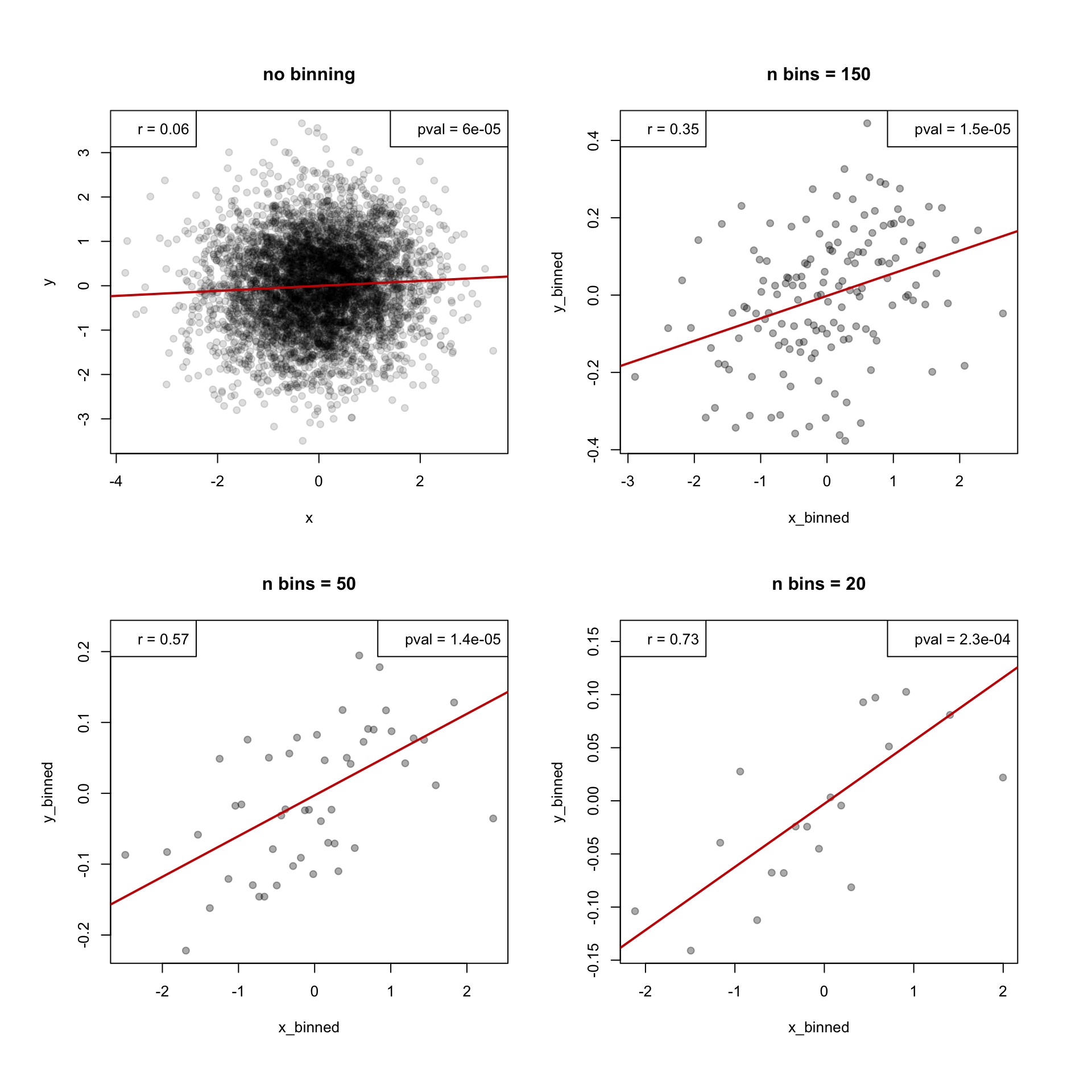
- using fewer bins (more data points in one bin) the correlation becomes greater
- p-value changed slightly
- note that axis ranges are different (it makes slopes look also different)
par(mfrow=c(2,2), oma=c(2,2,2,2))

# plot without binning
plot(y ~ x, data = df, main = "no binning", pch=19, col = "#00000022", xlim = c(-4,4), ylim = c(-4,4))
legend("topleft", legend = paste("r =", round(cor(df$x,df$y),2)))
legend("topright", legend = paste("pval =", format(cor.test(df$x,df$y)$p.value, digits = 2, scientific = T)))
abline(lm(y ~x, data = df), col="red3", lwd=2)


# iterate through different number of bins
for(n_bins in c(150,50,20)){
    x_binned <- sapply(1:n_bins, FUN = function(i){  mean(df$x[((i-1)*(n/n_bins)+1):((i)*(n/n_bins))])})
    y_binned <- sapply(1:n_bins, FUN = function(i){  mean(df$y[((i-1)*(n/n_bins)+1):((i)*(n/n_bins))])})

    plot(x_binned, y_binned, main = paste("n bins =", n_bins), pch=19, col = "#00000055", xlim = c(-4,4), ylim = c(-4,4))
    legend("topleft", legend = paste("r =", round(cor(x_binned,y_binned),2)))
    legend("topright", legend = paste("pval =", format(cor.test(x_binned,y_binned)$p.value, digits = 2, scientific = T)))
    abline(lm(y_binned ~ x_binned), col="red3", lwd=2)
}

- slopes are actually similar